Полезное:
Как сделать разговор полезным и приятным
Как сделать объемную звезду своими руками
Как сделать то, что делать не хочется?
Как сделать погремушку
Как сделать так чтобы женщины сами знакомились с вами
Как сделать идею коммерческой
Как сделать хорошую растяжку ног?
Как сделать наш разум здоровым?
Как сделать, чтобы люди обманывали меньше
Вопрос 4. Как сделать так, чтобы вас уважали и ценили?
Как сделать лучше себе и другим людям
Как сделать свидание интересным?

Категории:
АрхитектураАстрономияБиологияГеографияГеологияИнформатикаИскусствоИсторияКулинарияКультураМаркетингМатематикаМедицинаМенеджментОхрана трудаПравоПроизводствоПсихологияРелигияСоциологияСпортТехникаФизикаФилософияХимияЭкологияЭкономикаЭлектроника
Topic: Graphs
|
|
The Graph Abstract Data Type (Graph ADT) is a set of objects (graphs) plus set of operations on graphs. Here we shall discuss only graph objects and some graph-related terms used in this book. The graph terminology is vast and not finally settled. Graph operations discussed in this book solve specific problems presented in graph terms. Many practical problems are stated as graph problems. Solution of graph problems have generated numerous algorithmic ideas. Later chapters include some examples of graph problems and algorithms to solve them.
Informally, a graph G is a picture (graph diagram) consisting of points (vertices) and lines (edges). It is not important if lines are straight or curved, long or short. Edges may be directed or undirected which result in directed or undirected graphs.
Formally, a graph G = <VG, EG> is a pair of sets, where VG = {v1, v2,…, vn,} is a set of vertices and EG = {e1, e2,…, em,} is a set of edges. Each edge is a pair of some vertices:
- ei = { vj , vk } is an unordered pair if ei is an undirected edge;
- ei = (vj , vk ) is an ordered pair if ei is a directed edge that begins in vj (edge tail) and ends in vk (edge head).

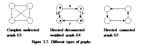
Vertex vj is adjacent to vertex vk if vk can be reached from vj through one edge. So in an undirected edge {vj , vk} both vertices are adjacent to each other. In a directed edge (vj , vk) only vk is adjacent to vj. For example, in G1 both B and C are adjacent, B and D are not adjacent. In the graph G4, A is adjacent to B but the opposite is wrong.
A pathfrom vertex vj to vertex vk is a sequence of edges that connects vj and vk in a graph. In a path of a directed graph the head of each previous edge is equal to the tail in each next edge (edges have the same direction). For example, in G1 {B, C}, {C, A}, {A, D} is one of the paths from B to D. In G4 the directed sequence (B, C), (C, D), (D, A) is a path that connects B to A. The sequence (B, A), (D, A) is not a path.
A cycle is a path that begins and ends in the same vertex. For example, in G1 {B, C}, {C, A}, {A, B} is one of the cycles. In G4 there are no cycles. Such a graph is called acyclic.
The degree (degree(vj)) of a vertex vj is the number of vertices adjacent to vj in a graph. For example, in G1 degree(B) = 2 and degree(A) = 3. In G4 degree(B) = 2 and degree(A) = 0.
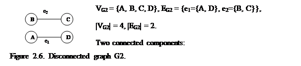
A graph is called connected if any two vertices in it are connected by an edge or a path. Otherwise, a graph is disconnected. For example, G1 and G5 are connected graphs. G2 and G4 are disconnected graphs.
Graph S = <VS, ES> is called a subgraph of graph G = <VG, EG> if VS ÍVG and ES ÍEG . For example, in graph G2 there are only two connected subgraphs. Other subgraphs of G2 are just isolated vertices. In G1 the subsets {A, B, C} and {e1, e2} can be treated as a subgraph of G1. G1 contains other subgraphs also.
A maximum connected subgraph of G is called itsconnected component.
A graph is called complete if any two vertices are connected by an edge. An undirected complete graph of n vertices contains the maximum number of edges which is equal to

In an empty graph, the set of vertices is empty.
A graph is called sparse if the number of its edges is closer to 0 than to the maximum number.
In a dense graph the number of edges is closer to the maximum number than to 0. For example, G1 is a dense graph and G2 is a sparse graph.
In a weighted graph G = <V, E, W>, edges are assigned numbers (weights, costs, lengths). W is a set of weights of edges.
There are two main methods for representing graphs in computer memory. Usually a dense graph G is represented by its adjacency matrix AG = (aij) which is a square matrix with rows and columns corresponding to vertices. Elements aij of such a matrix are specified differently depending on the type of a graph.
For an unweighted graph (directed or undirected), an element aij is defined so:
if vertex vi is adjacent to vertex vj then aij =1; otherwise aij= 0.
In case of a weighted graph (directed or undirected), element aij is defined so:
if vi is adjacent to vj then aij = weight of the edge; otherwise aij= ¥.
For an undirected graph (weighted or unweighted), its adjacency matrix is symmetrical against the main diagonal. So only half of its elements (below or above the main diagonal) may be actually entered in computer memory.
For a directed graph (weighted or unweighted), its adjacency matrix is not symmetrical. So all its elements must be entered in computer memory.
For example, the adjacency matrices for graphs G1 and G4 look as follows:
| i \ j | A | B | C | D | i \ j | A | B | C | D | |||||
| A | A | ¥ | ¥ | ¥ | ¥ | |||||||||
| AG1= | B | AG4= | B | ¥ | ¥ | |||||||||
| C | C | ¥ | ¥ | ¥ | ||||||||||
| D | D | ¥ | ¥ | ¥ |
Figure 2.8. Adjacency matrices for graph G1 and directed weighted graph G4.
A graph can be presented in computer memory by an array of adjacency lists (adjacency lists).Elementsof such an array are indexed by vertices. Each array element #j contains a pointer (reference) at a list of vertices adjacent to vertex vj. (an adjacency list for vj). Typically each adjacency list is a linked list with pointers (references) to dynamic memory.
In the following examples, the symbol ‘Æ’ denotes NULL pointer (null reference).
| A | 
| B |
| C | 
| D | Æ | A | Æ | |||||||||||||
| B | 
| A |
| C | Æ | B | 
| A | 
| C | Æ | |||||||||||
| C |
| A |
| B |
| D | Æ | C |
| D | Æ | |||||||||||
| D |
| A |
| C | Æ | D |
| A | Æ |
Figure 2.9. Adjacency lists for G1. Figure 2.10. Adjacency lists for G4
Representation of a graph G = <VG, EG> by its adjacency lists requires time and memory both in O(|EG|). That is why it is more efficient for sparse graphs.
A graph can be formally represented by many other methods. We shall discuss some of these methods when they are required by an algorithm. The operation of a graph algorithm is greatly influenced by the method of the graph representation.
Trees
Trees are special types of graphs. Tree vertices are often called nodes.
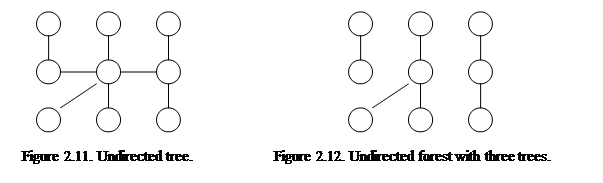
An undirected tree (tree) is an undirected connected acyclic graph.
An undirected forest is an undirected disconnected acyclic graph. Connected components of a forest are trees.
An undirected tree may represent:
- a map of two-way highways connecting towns;
- a molecular structure;
- an electrical circuit, etc.
Here are some features of any undirected tree T = <VT, ET>:
- |VT| = |ET| +1.
- Any two nodes are connected by a single path.
- If any edge is removed from T then T becomes disconnected.
- If any edge is added to T then T contains exactly one cycle.
A rooted tree is a directed tree with a special node called the root. The tree root is the node that appears first, gives the origin to other nodes in tree. In a rooted tree, the tail of every directed edge is called father node and the head is called son node.
A binary tree is a rooted tree where every father node has not more than two son nodes.
Most algorithms for binary trees are recursive since the nature of a binary tree itself is also recursive. A binary tree is a finite set of nodes which is either empty or is partitioned into three disjoined subsets:
- a single node called the root;
- a subset of nodes called the left subtree which is a binary tree itself;
- a subset of nodes called the right subtree which is a binary tree itself.

In the tree T1, the root node a is the father for three son nodes: b, c, d. The node c has no son nodes (its degree is equal 0). In a tree, a node with no son nodes is called a leaf. T1 contains such leaves: c, e, f, g.
In the binary tree T2, the direction of edges is not specified. In any binary tree, edges are assumed to be directed down from its root to leaves. T2 can be specified as a general graph: T2 = < VT2 = {h, i, j, k, l}, VT2 ={(h, i), (h, j), (i, k), (i, l)}>.
The binary tree T2 can be specified recursively so:
T2 = {root1 = {h}, left subtree1 = {i, k, l}, right subtree1 = {j}};
left subtree1 = { root2 = {i}, left subtree2 = (k}, right subtree2 = {l}};
right subtree1 = {root3 = {j}, left subtree3 = {Ø}, right subtree3 = {Ø}};
left subtree2 = {root4 = {k}, left subtree4 = {Ø}, right subtree4 = {Ø}};
right subtree2 = {root5 = {l}, left subtree5 = {Ø}, right subtree5 = {Ø}};
In a binary tree the level of a node is defined as the length of the path from the tree root to the node. In T2 the node h (the root) belongs to level #0, nodes i and j fit in level #1, finally k and l are at level #2.
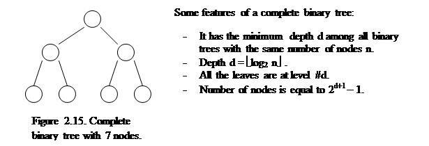
The maximum level of a node in a binary tree is called the depth (the height) of the binary tree. The depth of T2 is 2.
A binary tree with exactly 2level nodes at each level is called a complete (full) binary tree, where level = 0, 1, …, depth.
A method of representation in memory depends on the tree type and the algorithm for processing the tree. A general tree (directed or undirected) can be represented as any graph: by its adjacency matrix, list of adjacencies, etc.
A binary tree is often represented by dynamic nodes linked via pointers (references). For example, the memory representation of the binary tree T2 (Figure 2.14) can be viewed so:
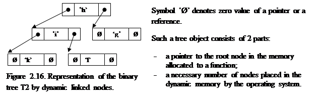
This method is preferable if a binary tree is processed by some recursive algorithm because each node is a root of some binary tree. Such a representation requires some extra memory for pointers. Not all algorithms for binary trees are recursive. That is why other methods are also used for representing binary trees. For example, a heap (a special type a binary tree) is conveniently presented by an array. We shall discuss this method later in relation to heapsort.
Date: 2015-12-11; view: 761; Нарушение авторских прав